当前位置：首页 > article >正文

第T7周：咖啡豆识别

article 2024/10/25 3:20:48

>- **🍨 本文为[🔗365天深度学习训练营](https://mp.weixin.qq.com/s/0dvHCaOoFnW8SCp3JpzKxg) 中的学习记录博客**
>- **🍖 原作者：[K同学啊](https://mtyjkh.blog.csdn.net/)**
难度：夯实基础⭐⭐
语言：Python3、TensorFlow2
🏡 我的环境：
语言环境：Python3.8
编译器：jupyter lab
深度学习环境：TensorFlow2.4.1

一、前期工作

1. 设置GPU

如果使用的是CPU可以忽略这步

import tensorflow as tf

gpus = tf.config.list_physical_devices("GPU")

if gpus:
    tf.config.experimental.set_memory_growth(gpus[0], True)  #设置GPU显存用量按需使用
    tf.config.set_visible_devices([gpus[0]],"GPU")

2. 导入数据

from tensorflow       import keras
from tensorflow.keras import layers,models
import numpy             as np
import matplotlib.pyplot as plt
import os,PIL,pathlib

data_dir = "./49-data/"
data_dir = pathlib.Path(data_dir)

image_count = len(list(data_dir.glob('*/*.png')))

print("图片总数为：",image_count)

1200

二、数据预处理

1. 加载数据

使用image_dataset_from_directory方法将磁盘中的数据加载到tf.data.Dataset中

from tensorflow import keras
from tensorflow.keras import layers, models
import os, PIL, pathlib
import matplotlib.pyplot as plt
import tensorflow as tf
import numpy as np
import tensorflow as tf

batch_size = 32
img_height = 224
img_width = 224
train_ds = tf.keras.preprocessing.image_dataset_from_directory(
    data_dir,
    validation_split=0.2,
    subset="training",
    seed = 123,
    image_size=(img_height, img_width),
    batch_size=batch_size
)
val_ds = tf.keras.preprocessing.image_dataset_from_directory(
    data_dir,
    validation_split=0.2,
    subset="validation",
    seed = 123,
    image_size=(img_height, img_width),
    batch_size=batch_size
)
class_names = train_ds.class_names
print(class_names)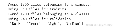

2. 可视化数据

plt.figure(figsize=(10,4))
for images, labels in train_ds.take(1):
    for i in range(10):
        ax = plt.subplot(2, 5, i+1)
        plt.imshow(images[i].numpy().astype('uint8'))
        plt.title(class_names[np.argmax(labels[i])])
        
        plt.axis('off')
for image_batch, labels_batch in train_ds:
    print(image_batch.shape) 
    print(labels_batch.shape)
    break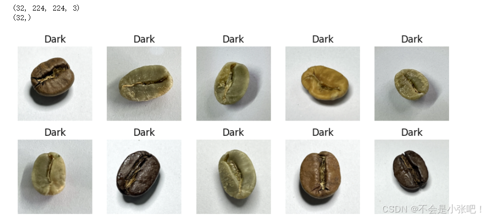

3. 配置数据集

AUTOTUNE = tf.data.AUTOTUNE
 
train_ds = train_ds.cache().shuffle(1000).prefetch(buffer_size = AUTOTUNE)
val_ds = val_ds.cache().prefetch(buffer_size=AUTOTUNE)
normalization_layer = layers.experimental.preprocessing.Rescaling(1./255)
 
train_ds = train_ds.map(lambda x, y: (normalization_layer(x), y))
val_ds   = val_ds.map(lambda x, y: (normalization_layer(x), y))
image_batch, labels_batch = next(iter(val_ds))
first_image = image_batch[0]
print(np.min(first_image), np.max(first_image))

0.0 1.0

三、构建VGG-16网络

在官方模型与自建模型之间进行二选一就可以了，选着一个注释掉另外一个。

VGG优缺点分析：

VGG优点

VGG的结构非常简洁，整个网络都使用了同样大小的卷积核尺寸（3x3）和最大池化尺寸（2x2）。

VGG缺点

1)训练时间过长，调参难度大。2)需要的存储容量大，不利于部署。例如存储VGG-16权重值文件的大小为500多MB，不利于安装到嵌入式系统中。

自建模型

from tensorflow.keras import layers, models, Input
from tensorflow.keras.models import Model
from tensorflow.keras.layers import Conv2D, MaxPooling2D, Dense, Flatten, Dropout
 
def VGG16(nb_classes, input_shape):
    input_tensor = Input(shape=input_shape)
    # 1st block
    x = Conv2D(64, (3,3), activation='relu', padding='same',name='block1_conv1')(input_tensor)
    x = Conv2D(64, (3,3), activation='relu', padding='same',name='block1_conv2')(x)
    x = MaxPooling2D((2,2), strides=(2,2), name = 'block1_pool')(x)
    # 2nd block
    x = Conv2D(128, (3,3), activation='relu', padding='same',name='block2_conv1')(x)
    x = Conv2D(128, (3,3), activation='relu', padding='same',name='block2_conv2')(x)
    x = MaxPooling2D((2,2), strides=(2,2), name = 'block2_pool')(x)
    # 3rd block
    x = Conv2D(256, (3,3), activation='relu', padding='same',name='block3_conv1')(x)
    x = Conv2D(256, (3,3), activation='relu', padding='same',name='block3_conv2')(x)
    x = Conv2D(256, (3,3), activation='relu', padding='same',name='block3_conv3')(x)
    x = MaxPooling2D((2,2), strides=(2,2), name = 'block3_pool')(x)
    # 4th block
    x = Conv2D(512, (3,3), activation='relu', padding='same',name='block4_conv1')(x)
    x = Conv2D(512, (3,3), activation='relu', padding='same',name='block4_conv2')(x)
    x = Conv2D(512, (3,3), activation='relu', padding='same',name='block4_conv3')(x)
    x = MaxPooling2D((2,2), strides=(2,2), name = 'block4_pool')(x)
    # 5th block
    x = Conv2D(512, (3,3), activation='relu', padding='same',name='block5_conv1')(x)
    x = Conv2D(512, (3,3), activation='relu', padding='same',name='block5_conv2')(x)
    x = Conv2D(512, (3,3), activation='relu', padding='same',name='block5_conv3')(x)
    x = MaxPooling2D((2,2), strides=(2,2), name = 'block5_pool')(x)
    # full connection
    x = Flatten()(x)
    x = Dense(4096, activation='relu',  name='fc1')(x)
    x = Dense(4096, activation='relu', name='fc2')(x)
    output_tensor = Dense(nb_classes, activation='softmax', name='predictions')(x)
 
    model = Model(input_tensor, output_tensor)
    return model
 
model=VGG16(len(class_names), (img_width, img_height, 3))
model.summary()

四、编译

在准备对模型进行训练之前，还需要再对其进行一些设置。以下内容是在模型的编译步骤中添加的：
●损失函数（loss）：用于衡量模型在训练期间的准确率。
●优化器（optimizer）：决定模型如何根据其看到的数据和自身的损失函数进行更新。
●指标（metrics）：用于监控训练和测试步骤。以下示例使用了准确率，即被正确分类的图像的比率。

# 设置初始学习率
initial_learning_rate = 1e-4
 
lr_schedule = tf.keras.optimizers.schedules.ExponentialDecay(
        initial_learning_rate, 
        decay_steps=30,      
        decay_rate=0.92,     
        staircase=True)
 
# 设置优化器
opt = tf.keras.optimizers.Adam(learning_rate=initial_learning_rate)
 
model.compile(optimizer=opt,
              loss=tf.keras.losses.SparseCategoricalCrossentropy(from_logits=True),
              metrics=['accuracy'])

五、训练模型

🔊注：从本周开始，网络越来越复杂，对算力要求也更高，CPU训练模型时间会很长，建议尽可能的使用GPU来跑。

epochs = 20

history = model.fit(
    train_ds,
    validation_data=val_ds,
    epochs=epochs
)

六、可视化结果

acc = history.history['accuracy']
val_acc = history.history['val_accuracy']
 
loss = history.history['loss']
val_loss = history.history['val_loss']
 
epochs_range = range(epochs)
 
plt.figure(figsize=(12, 4))
plt.subplot(1, 2, 1)
plt.plot(epochs_range, acc, label='Training Accuracy')
plt.plot(epochs_range, val_acc, label='Validation Accuracy')
plt.legend(loc='lower right')
plt.title('Training and Validation Accuracy')
 
plt.subplot(1, 2, 2)
plt.plot(epochs_range, loss, label='Training Loss')
plt.plot(epochs_range, val_loss, label='Validation Loss')
plt.legend(loc='upper right')
plt.title('Training and Validation Loss')
plt.show()