机器学习（10.14-10.20）(Pytorch GRU的原理及其手写复现)

摘要

GRU是RNN的一个优秀的变种模型，继承了大部分RNN模型的特性；在本次学习中，简单学习了GRU的基础知识，展示了GRU的手动推导过程，用代码逐行模拟实现LSTM的运算过程，并与Pytorch API输出的结验证是否保持一致。

Abstract

GRU is an excellent variant model of RNN, inheriting most of the characteristics of RNN model. In this study, I simply learned the basic knowledge of GRU, demonstrated the manual derivation process of GRU, simulated the operation process of LSTM with code line by line, and verified whether it was consistent with the junction output of Pytorch API.

GRU

GRU（Gate Recurrent Unit）门控循环单元，是循环神经网络(RNN)的变种，与LSTM类似通过门控单元解决RNN中不能长期记忆和反向传播中的梯度等问题。与LSTM相比，GRU内部的网络架构较为简单。

1.1 GRU网络的基本结构

GRU 网络内部包含两个门使用了更新门（update gate）与重置门（reset gate）。重置门决定了如何将新的输入信息与前面的记忆相结合，更新门定义了前面记忆保存到当前时间步的量。如果我们将重置门设置为 1，更新门设置为 0，那么我们将再次获得标准 RNN 模型。这两个门控向量决定了哪些信息最终能作为门控循环单元的输出。这两个门控机制的特殊之处在于，它们能够保存长期序列中的信息，且不会随时间而清除或因为与预测不相关而移除。 GRU门控结构如下图所示:

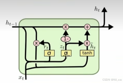
1. 重置门：
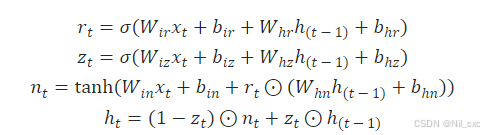
   重置门（reset gate），记为$r_t$，这个门决定了上一时间步的记忆状态如何影响当前时间步的候选记忆内容。计算时会结合前一时间步的隐藏状态$h_{t-1}和x_t$，输出是一个0到1之间的值。值越接近1表示越多地保留之前的状态，越接近0表示遗忘更多旧状态。对应的数学表达如下：

$$r_t=\sigma (Wr\ast [h_{t-1},x_t])$$

2. 更新门：
   更新门（update gate），记为$z_t$，这个门决定了上一时间步的记忆状态有多少需要传递到当前时间步，以及当前的输入信息有多少需要加入到新的记忆状态中，同样，它也是基于前一时间步的隐藏状态$h_{t-1}和x_t$计算得到的。对应的数学表达如下：
   $$z_t=\sigma (Wz\ast [h_{t-1},x_t])$$

3. 候选记忆状态：
   候选记忆状态，记为${\tilde{h}}_t$，基于当前输入$x_t$和上一时间步隐藏状态$h_{t-1}$以及重置门的输出，三者计算得到的，其中的重置门决定了如何“重置”旧的记忆状态，以便更好地整合新信息。对应的数学表达如下：
   $${\tilde{h}}_t=tanh(W\cdot [r_t\ast h_{t-1},x_t])$$

4. 最终记忆状态：
   最终记忆状态，记为$h_t$,通过结合更新门的输出和候选记忆状态以及上一时间步的记忆状态来计算得出的。其中更新门决定了新旧记忆的混合比例。对应的数学表达如下：
   $$h_t=(1-z_t)\ast h_{t-1}+z_t\ast {\tilde{h}}_t$$

1.2 举个例子说明GRU的工作原理

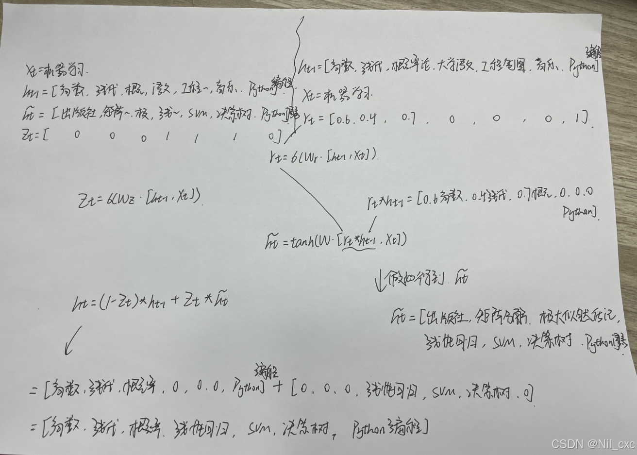
我们可以把某个学生的学习历程想象成一个时间序列，其中每个学科对应一个时间步骤上的输入数据。每个笔记代表了在特定时间点（假设从小学、初中、高中到大学）学习的内容。我们想利用GRU模型来理解学生的学习轨迹。

在t-1时刻我们有[高数，线代，概率论，。。。]这些笔记存放在书柜中，在t时刻我们要进行学习机器学习，但是我们的书柜空间有限，我们就要把跟机器学习不相关的笔记清理掉，把新的笔记加入到里面

1. 重置门：$r_t$的值，是去筛选那些笔记内容跟学习机器学习相关联的内容，例：高数有60%帮助我们学习机器学习等等。
2. 更新门：$z_t$的值，决定了上一时间步的记忆状态有多少需要传递到当前时间步，以及当前的候选记忆状态中有多少需要加入到新的记忆状态中
3. 候选记忆状态${\tilde{h}}_t$，经过重置门过滤后，之前的知识和新的输入共同决定了新的候选隐藏状态。以此模拟学生如何将过去的知识与新知识结合起来。
4. 最终隐藏状态：更新门负责把新的候选隐藏状态与旧的隐藏状态结合起来，创造出最新的隐藏状态，代表学生整合了新旧知识后的当前知识水平。

1.3 使用Pytorch GRU

实例化GRU类，需要传递的参数：

input_size：输入数据的特征维度
hidden_size：隐含状态$h_t$的大小
num_layers：默认值为1，大于1，表示多个RNN堆叠起来
batch_first：默认是False；若为True,输入输出格式为：(batch, seq, feature) ；若为False：输入输出格式为： (seq, batch, feature)；
bidirectional：默认为False；若为True，则是双向GRU，同时输出长度为2*hidden_size

函数输入值：（input，h_0）

1. input：当batch_first=True 输入格式为（N,L,$H_{in}$）;当batch_first=False 输入格式为（L,N,$H_{in}$）;
2. h_0：默认输入值为0；输入格式为：（D*num_layers,N,$H_{out}$）

其中：

N = batch size
L = sequence length
D = 2 if bidirectional=True otherwise 1
$H_{in}$ = input_size
$H_{out}$ = hidden_size

函数输出值：（output，h_n）

1. output：当batch_first=True 输出格式为（N，L，D*$H_{out}$）;当batch_first=False 输出格式为（L，N，D*$H_{out}$）;
2. h_n：输出格式为：（D*num_layers，N，$H_{out}$）

首先实例化一些参数：

# 初始化参数
bs, T, input_size, hidden_size = 2, 3, 4, 5
input = torch.randn(bs, T, input_size)
h0 = torch.randn(bs, hidden_size)

调用Pytorch中的GRU API:
并查看返回的结果及其形状

# 官方GRU API
gru = nn.GRU(input_size, hidden_size, batch_first=True)
output, h_n = gru(input, h0.unsqueeze(0))
print(output)
print(output.shape) # torch.Size([2, 3, 5])
print(h_n)
print(h_n.shape)    # torch.Size([1, 2, 5])

输出为：

tensor([[[ 0.9957, -2.1179,  1.8409, -0.3901, -0.0735],
         [ 0.3356, -1.1755,  1.4708, -0.2688,  0.1032],
         [ 0.0467, -0.8454,  1.1640, -0.1547,  0.2743]],

        [[-0.2165, -1.1894,  0.1635, -0.5871,  0.0576],
         [-0.3580, -0.7435,  0.0280, -0.1813, -0.0567],
         [-0.1103, -0.3540,  0.5457, -0.4038, -0.3709]]],
       grad_fn=<TransposeBackward1>)
torch.Size([2, 3, 5])
tensor([[[ 0.0467, -0.8454,  1.1640, -0.1547,  0.2743],
         [-0.1103, -0.3540,  0.5457, -0.4038, -0.3709]]],
       grad_fn=<StackBackward0>)
torch.Size([1, 2, 5])

1.4 手写实现gru_forward函数 实现单向GRU的计算原理

def gru_forward(input, initial_state, w_ih, w_hh, b_ih, b_hh):
    bs, T, input_size = input.shape
    prev_h = initial_state
    hidden_size = w_ih.shape[0] // 3

    # w_ih [3* hidden_size, input_size]  w_hh [3* hidden_size, hidden_size]
    batch_w_ih = w_ih.unsqueeze(0).tile(bs, 1, 1)   # [bs,3* hidden_size, input_size]
    batch_w_hh = w_hh.unsqueeze(0).tile(bs, 1, 1)   # [bs,3* hidden_size, hidden_size]

    output_size = hidden_size
    output = torch.zeros(bs, T, output_size)

    for t in range(T):
        x = input[:, t, :]  # [bs, input_size]

        # 矩阵运算
        # x: [bs, input_size] -> [bs, input_size,1]
        # w_ih : [bs, 3* hidden_size, input_size]
        x_times = torch.bmm(batch_w_ih, x.unsqueeze(-1)).squeeze(-1)    # [bs,3* hidden_size,1]->[bs,3* hidden_size]
        h_times = torch.bmm(batch_w_hh, prev_h.unsqueeze(-1)).squeeze(-1)   # [bs,3* hidden_size,1]->[bs,3* hidden_size]

        # 计算重置门的值：
        r_t = torch.sigmoid(x_times[:, :hidden_size] + h_times[:, :hidden_size] + b_ih[:hidden_size] + b_hh[:hidden_size])
        # 计算更新门的值：5
        z_t = torch.sigmoid(x_times[:, hidden_size:2*hidden_size] + h_times[:, hidden_size:2*hidden_size] +
                            b_ih[hidden_size:2*hidden_size] + b_hh[hidden_size:2*hidden_size])

        n_t = torch.tanh(x_times[:, 2*hidden_size:3*hidden_size]+b_ih[2*hidden_size:3*hidden_size] +
                         r_t*(h_times[:, 2*hidden_size:3*hidden_size]+b_hh[2*hidden_size:3*hidden_size]))
        prev_h = (1-z_t)*n_t + z_t*prev_h

        output[:, t, :] = prev_h

    return output, prev_h

获取 pytorch GRU内置参数

for k, v in gru.named_parameters():
    print(k, v.shape)

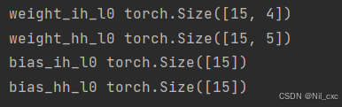
使用pytorch中GRU的内置参数测试该函数

c_output, c_hn = gru_forward(input, h0, gru.weight_ih_l0, gru.weight_hh_l0, gru.bias_ih_l0, gru.bias_hh_l0)
print(c_output)

print(torch.allclose(output, c_output))
print(torch.allclose(h_n, c_hn))

查看两者的输出结果完全相同

总结

在本次学习中，通过对GRU运算过程的代码逐行实现，了解到GRU模型，以及加深了自己对GRU模型的理解与推导。对于接下来的学习，我将对RNN,LSTM以及GRU三者的优缺点进行补充学习。