Merlion笔记(四):添加一个新的预测模型
文章目录
- 1 模型配置类
- 2 模型类
- 3 运行模型:一个简单的例子
- 4 可视化
- 5 定量评估
- 6 定义一个基于预测器的异常检测器
本文提供了一个示例,展示如何向 Merlion 添加一个新的预测模型,遵循 CONTRIBUTING.md 中的说明。建议在阅读本篇文章之前,先查看该 文章,了解如何使用 Merlion 的进行预测。
本文将实现一个预测模型,其预测值正好等于该时间点的前一个观测值。有关更真实的示例,请参阅对 Sarima 的实现。
1 模型配置类
创建新模型的第一步是定义一个配置类,该类继承自 ForecasterConfig:
from merlion.models.forecast.base import ForecasterConfig

class RepeatRecentConfig(ForecasterConfig):
    def __init__(self, max_forecast_steps=None, **kwargs):
        super().__init__(max_forecast_steps=max_forecast_steps, **kwargs)
2 模型类
接下来,定义模型本身,该模型必须继承自 ForecasterBase 基类,并实现所有抽象方法。
from collections import OrderedDict
from typing import List, Tuple

import numpy as np
import pandas as pd

from merlion.models.forecast.base import ForecasterBase
from merlion.utils.time_series import to_pd_datetime


class RepeatRecent(ForecasterBase):
    # RepeatRecent 的配置类是上面定义的 RepeatRecentConfig
    config_class = RepeatRecentConfig

    @property
    def require_even_sampling(self):
        """
        许多预测模型假设输入的时间序列是均匀采样的。这个模型不需要这种假设,因此重写该属性。
        """
        return False

    def __init__(self, config):
        """
        设置模型配置和其他局部变量。在这里,我们将 most_recent_value 初始化为 None。
        """
        super().__init__(config)
        self.most_recent_value = None


    def _train(self, train_data: pd.DataFrame, train_config=None) -> Tuple[pd.DataFrame, None]:
        # 训练模型。在这里,我们只是收集每个单变量的最新观察值。
        # 列表推导式,用来遍历 train_data 的每一列(键值对形式)。对于每一列,k 是列名,v.values[-1]
        # 是该列的最后一个观测值。最终生成一个列表,其中每个元素是 (列名, 最近观测值) 这样的元组。
        self.most_recent_value = [(k, v.values[-1]) for k, v in train_data.items()]

        # 模型的目标值是每个时间序列的前一个值,即每一行的预测值是上一时间点的实际值。
        # 将一个全 0 的数组与 train_data(去掉最后一行后的数据)拼接起来,形成一个新的数组 pred,这个数组的每一行都是前一个时间点的数值。
        pred = np.concatenate((np.zeros((1, self.dim)), train_data.values[:-1]))
        train_forecast = pd.DataFrame(pred, index=train_data.index, columns=train_data.columns)

        # 这个模型没有误差的概念
        train_stderr = None

        # 返回训练的预测结果和标准误差
        return train_forecast, train_stderr

    def _forecast(self, time_stamps: List[int], time_series_prev: pd.DataFrame = None, return_prev=False) -> Tuple[pd.DataFrame, None]:

        # 如果提供了 time_series_prev,则使用其最近的值。否则,使用从训练数据中存储的最近值
        if time_series_prev is not None:
            most_recent_value = [(k, v.values[-1]) for k, v in time_series_prev.items()]
        else:
            most_recent_value = self.most_recent_value

        # 预测值只是将最近的一个值重复用于每一个未来的时间点。
        i = self.target_seq_index # 目标序列的索引
        datetimes = to_pd_datetime(time_stamps) # 测试序列的时间戳
        name, val = most_recent_value[i]
        forecast = pd.DataFrame([val] * len(datetimes), index=datetimes, columns=[name])

        # 如果需要,给 time_series_prev 的 target_seq_index 预加上“预测”值。
        if return_prev and time_series_prev is not None:
            pred = np.concatenate(([0], time_series_prev.values[:-1, i]))
            prev_forecast = pd.DataFrame(pred, index=time_series_prev.index, columns=[name])
            forecast = pd.concat((prev_forecast, forecast))

        return forecast, None
3 运行模型:一个简单的例子
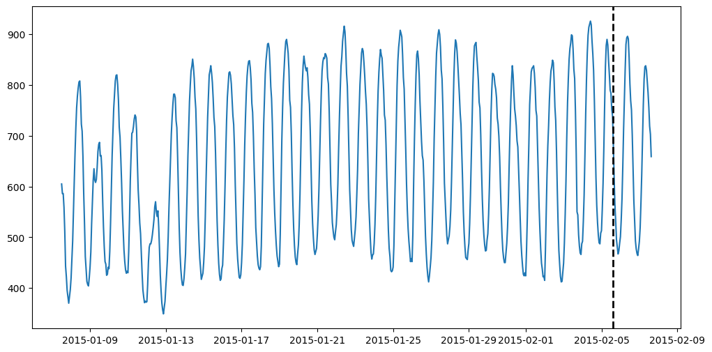
尝试在一些实际数据上运行这个模型!我们将首先从 M4 数据集中获取时间序列并将其可视化。
import matplotlib.pyplot as plt
import pandas as pd

from merlion.utils import TimeSeries, UnivariateTimeSeries
from ts_datasets.forecast import M4

time_series, metadata = M4(subset="Hourly")[0]

# Visualize the full time series
fig = plt.figure(figsize=(12, 6))
ax = fig.add_subplot(111)
ax.plot(time_series)

# Label the train/test split with a dashed line
ax.axvline(time_series[metadata["trainval"]].index[-1], ls="--", lw=2, c="k")

plt.show()
现在,将数据分成训练和测试部分,并在其上运行我们的预测模型。
train_data = TimeSeries.from_pd(time_series[metadata["trainval"]])
test_data = TimeSeries.from_pd(time_series[~metadata["trainval"]])
# Initialize a model & train it. The dataframe returned & printed
# below is the model's "forecast" on the training data. None is
# the uncertainty estimate.
model = RepeatRecent(RepeatRecentConfig())
model.train(train_data=train_data)
(                        H1
 time
 2015-01-07 12:00:00    0.0
 2015-01-07 13:00:00  605.0
 2015-01-07 14:00:00  586.0
 2015-01-07 15:00:00  586.0
 2015-01-07 16:00:00  559.0
 ...                    ...
 2015-02-05 11:00:00  820.0
 2015-02-05 12:00:00  790.0
 2015-02-05 13:00:00  784.0
 2015-02-05 14:00:00  752.0
 2015-02-05 15:00:00  739.0

 [700 rows x 1 columns],
 None)
# Let's run our model on the test data now
forecast, err = model.forecast(test_data.to_pd().index)
print("Forecast")
print(forecast)
print()
print("Error")
print(err)
Forecast
                        H1
time
2015-02-05 16:00:00  684.0
2015-02-05 17:00:00  684.0
2015-02-05 18:00:00  684.0
2015-02-05 19:00:00  684.0
2015-02-05 20:00:00  684.0
2015-02-05 21:00:00  684.0
2015-02-05 22:00:00  684.0
2015-02-05 23:00:00  684.0
2015-02-06 00:00:00  684.0
2015-02-06 01:00:00  684.0
2015-02-06 02:00:00  684.0
2015-02-06 03:00:00  684.0
2015-02-06 04:00:00  684.0
2015-02-06 05:00:00  684.0
2015-02-06 06:00:00  684.0
2015-02-06 07:00:00  684.0
2015-02-06 08:00:00  684.0
2015-02-06 09:00:00  684.0
2015-02-06 10:00:00  684.0
2015-02-06 11:00:00  684.0
2015-02-06 12:00:00  684.0
2015-02-06 13:00:00  684.0
2015-02-06 14:00:00  684.0
2015-02-06 15:00:00  684.0
2015-02-06 16:00:00  684.0
2015-02-06 17:00:00  684.0
2015-02-06 18:00:00  684.0
2015-02-06 19:00:00  684.0
2015-02-06 20:00:00  684.0
2015-02-06 21:00:00  684.0
2015-02-06 22:00:00  684.0
2015-02-06 23:00:00  684.0
2015-02-07 00:00:00  684.0
2015-02-07 01:00:00  684.0
2015-02-07 02:00:00  684.0
2015-02-07 03:00:00  684.0
2015-02-07 04:00:00  684.0
2015-02-07 05:00:00  684.0
2015-02-07 06:00:00  684.0
2015-02-07 07:00:00  684.0
2015-02-07 08:00:00  684.0
2015-02-07 09:00:00  684.0
2015-02-07 10:00:00  684.0
2015-02-07 11:00:00  684.0
2015-02-07 12:00:00  684.0
2015-02-07 13:00:00  684.0
2015-02-07 14:00:00  684.0
2015-02-07 15:00:00  684.0

Error
None
4 可视化
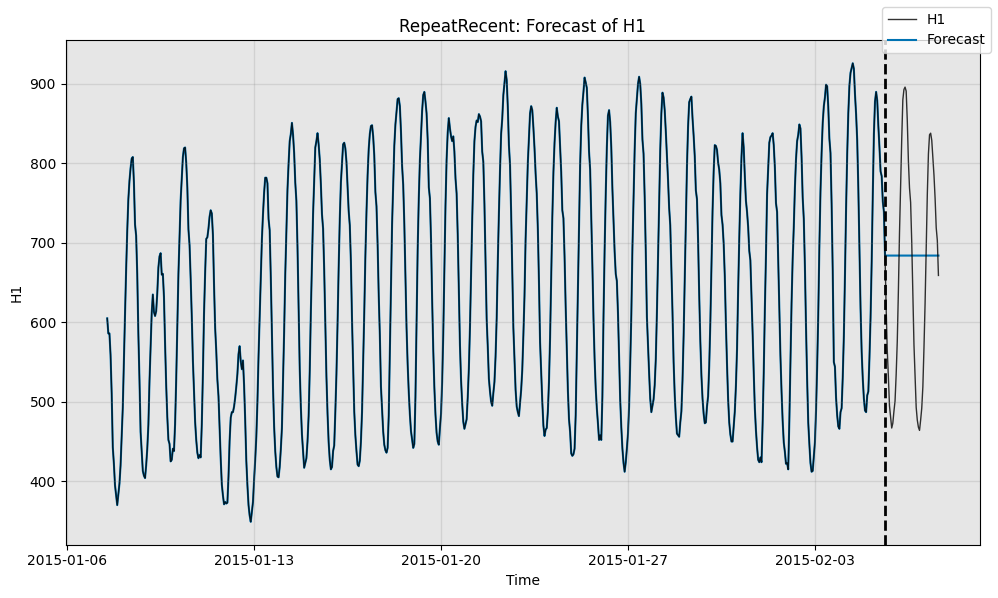
# Qualitatively, we can see what the forecaster is doing by plotting
print("Forecast w/ ground truth time series")
fig, ax = model.plot_forecast(time_series=test_data,
time_series_prev=train_data,
plot_time_series_prev=True)
plt.show()
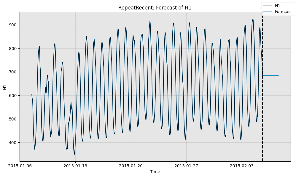
print()
print("Forecast without ground truth time series")
fig, ax = model.plot_forecast(time_stamps=test_data.to_pd().index,
time_series_prev=train_data,
plot_time_series_prev=True)
Forecast w/ ground truth time series
Forecast without ground truth time series
5 定量评估
也可以对模型进行定量评估。计算模型预测结果与真实数据的对称平均百分比误差(sMAPE,symmetric Mean Average Percent Error)。
from merlion.evaluate.forecast import ForecastMetric
smape = ForecastMetric.sMAPE.value(ground_truth=test_data, predict=forecast)
print(f"sMAPE = {smape:.3f}")
sMAPE = 20.166
6 定义一个基于预测器的异常检测器
将一个预测模型转换为异常检测模型是非常简单的。只需要在合适的目录下创建一个新文件,并定义包含一些基本头部的类结构。通过多重继承 ForecastingDetectorBase 类,大部分繁重的工作都可以自动处理。
任何基于预测的异常检测器返回的异常评分,都是基于预测值与真实时间序列值之间的残差。
from merlion.evaluate.anomaly import TSADMetric
from merlion.models.anomaly.forecast_based.base import ForecastingDetectorBase
from merlion.models.anomaly.base import DetectorConfig
from merlion.post_process.threshold import AggregateAlarms
from merlion.transform.normalize import MeanVarNormalize


# 定义一个配置类,该类按顺序继承自 RepeatRecentConfig 和 DetectorConfig
class RepeatRecentDetectorConfig(RepeatRecentConfig, DetectorConfig):
    # 设置一个默认的异常评分后处理规则
    _default_post_rule = AggregateAlarms(alm_threshold=3.0)

    # 默认的数据预处理变换是均值-方差归一化,
    # 这样异常评分大致与 z-score 对齐
    _default_transform = MeanVarNormalize()

# 定义一个模型类,该类按顺序继承自 ForecastingDetectorBase 和 RepeatRecent
class RepeatRecentDetector(ForecastingDetectorBase, RepeatRecent):
    # 我们只需要设置配置类
    config_class = RepeatRecentDetectorConfig
# Train the anomaly detection variant
model2 = RepeatRecentDetector(RepeatRecentDetectorConfig())
model2.train(train_data)
                     anom_score
time
2015-01-07 12:00:00   -0.212986
2015-01-07 13:00:00   -0.120839
2015-01-07 14:00:00    0.000000
2015-01-07 15:00:00   -0.171719
2015-01-07 16:00:00   -0.305278
...                         ...
2015-02-05 11:00:00   -0.190799
2015-02-05 12:00:00   -0.038160
2015-02-05 13:00:00   -0.203519
2015-02-05 14:00:00   -0.082679
2015-02-05 15:00:00   -0.349798

[700 rows x 1 columns]
# Obtain the anomaly detection variant's predictions on the test data
model2.get_anomaly_score(test_data)
                     anom_score
time
2015-02-05 16:00:00   -0.413397
2015-02-05 17:00:00   -0.756835
2015-02-05 18:00:00   -0.966714
2015-02-05 19:00:00   -1.202032
2015-02-05 20:00:00   -1.291072
2015-02-05 21:00:00   -1.380111
2015-02-05 22:00:00   -1.341952
2015-02-05 23:00:00   -1.246552
2015-02-06 00:00:00   -1.163873
2015-02-06 01:00:00   -0.953994
2015-02-06 02:00:00   -0.686876
2015-02-06 03:00:00   -0.286198
2015-02-06 04:00:00    0.178079
2015-02-06 05:00:00    0.559676
2015-02-06 06:00:00    0.928554
2015-02-06 07:00:00    1.246552
2015-02-06 08:00:00    1.329232
2015-02-06 09:00:00    1.348311
2015-02-06 10:00:00    1.316512
2015-02-06 11:00:00    1.081193
2015-02-06 12:00:00    0.756835
2015-02-06 13:00:00    0.540597
2015-02-06 14:00:00    0.426117
2015-02-06 15:00:00    0.108119
2015-02-06 16:00:00   -0.311638
2015-02-06 17:00:00   -0.712316
2015-02-06 18:00:00   -0.966714
2015-02-06 19:00:00   -1.214752
2015-02-06 20:00:00   -1.316512
2015-02-06 21:00:00   -1.373751
2015-02-06 22:00:00   -1.399191
2015-02-06 23:00:00   -1.316512
2015-02-07 00:00:00   -1.221112
2015-02-07 01:00:00   -1.049393
2015-02-07 02:00:00   -0.737755
2015-02-07 03:00:00   -0.381598
2015-02-07 04:00:00    0.076320
2015-02-07 05:00:00    0.489717
2015-02-07 06:00:00    0.814075
2015-02-07 07:00:00    0.966714
2015-02-07 08:00:00    0.979434
2015-02-07 09:00:00    0.922194
2015-02-07 10:00:00    0.782275
2015-02-07 11:00:00    0.642356
2015-02-07 12:00:00    0.457917
2015-02-07 13:00:00    0.222599
2015-02-07 14:00:00    0.120839
2015-02-07 15:00:00   -0.158999
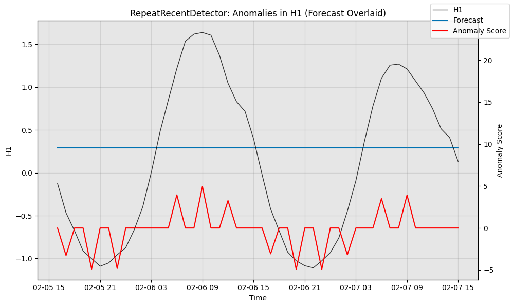
# Visualize the anomaly detection variant's performance, with filtered anomaly scores
fig, ax = model2.plot_anomaly(test_data, time_series_prev=train_data,
                              filter_scores=True, plot_time_series_prev=False,
                              plot_forecast=True)