当前位置：首页 > article >正文

随机模型预测控制（SMPC）——考虑概率约束（Matlab代码实现）

article 2025/2/25 9:06:18

💥1 概述

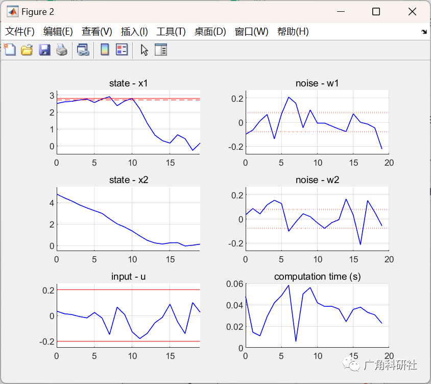
📚2 运行结果

🎉3 参考文献

👨‍💻4 Matlab代码

💥1 概述

模型预测控制（MPC）又称为滚动时域控制和滚动时域控制，是一种强有力的工程应用技术。MPC的价值主要体现在其处理约束的内在能力，同时最小化一些代价（或最大化一些回报）。MPC的基本思想是用有限时域最优控制问题来反复逼近无限时域约束最优控制问题。在每一个时间步，这样一个有限时域问题被解决，并且只有第一个输入以一种后退时域的方式被应用到系统中。

MPC使用一个对象模型来预测其未来的行为，然后根据预测计算出一个最优的输入轨迹。然而，在大多数实际应用中，由于模型的不确定性或外界干扰，都无法得到精确的模型。在文献中，不确定性通常是通过描述一个鲁棒MPC问题来解决的，在这个问题中，不确定性被假定为有界的，并且计算出满足每个可能的不确定性实现的约束的控制律。这种悲观的观点可能会显著降低控制器的整体性能，因为需要防范低概率不确定性异常值。

随机MPC（SMPC）提供了另一种对不确定性不那么悲观的观点。在SMPC中，约束是概率解释的，允许很小的违反概率。在这种情况下，甚至可以研究无界不确定性。不幸的是，SMPC问题通常很难解决，只能近似地或通过施加特定的问题结构来解决。在这种情况下，我们主要关注以下问题：但是如果不确定性没有界，会发生什么？或者当它不是均匀分布的时候？一个不太保守的方法显然是考虑到这些可能性，确定不确定性的适当分布，并制定一个随机的MPC问题。

📚2 运行结果

主函数部分代码：

% plot inputs and states 

%% run smpc (runs new MPC simulation)
[x,u, x1_limit, sig, beta, s, comp_time]= run_mpc;



%% plot input and states

% set up figure for input and states
figure(2)
clf

plot_noise = 1;         % plot noise? 0: no; 1: yes (if yes: computation time will also be plotted)
% if noise was not saved, automatically swich to 0
if exist('s','var') == 0
    plot_noise = 0;
end


steps = 0:length(x)-1;  % get steps (last input is computed but not applied) 


% state x1
if plot_noise == 0
    subplot(3,1,1)
else
    subplot(3,2,1)
end
hold on
title('state - x1')
grid on
plot(steps,x(:,1), 'b', 'Linewidth',0.8)
% plot constraint only if close enough
if x1_limit < 40
    yline(x1_limit, 'r', 'Linewidth',0.8)
    ylim([-0.5 x1_limit+0.5]);
    gamma1 = sqrt(2*[1;0]'*[sig^2 0; 0 sig^2]*[1;0])*erfinv(2*beta-1); % chance constraint addition for first predicted step
    yline(x1_limit-gamma1, 'r--', 'Linewidth',0.8)
end
xlim([steps(1) steps(end)]);
hold off


% state x2
if plot_noise == 0
    subplot(3,1,2)
else
    subplot(3,2,3)
end
hold on
title('state - x2')
plot(steps,x(:,2), 'b', 'Linewidth',0.8)
grid on
ylim([-0.5 5.5]);
xlim([steps(1) steps(end)]);
hold off


% input u
if plot_noise == 0
    subplot(3,1,3)
else
    subplot(3,2,5)
end
K = [0.2858 -0.4910];
u_applied = [];
for i = 1:length(u)
    u_applied(i,1) = u(i,1) - K*[x(i,1); x(i,2)];
end
hold on
title('input - u')
grid on
plot(steps,u_applied(:,1), 'b', 'Linewidth',0.8)
yline(0.2,'r', 'Linewidth',0.8)
yline(-0.2,'r', 'Linewidth',0.8)
ylim([-0.25 0.25]);
xlim([steps(1) steps(end)]);
hold off


% plot noise (given seeding)
% rng(30,'twister'); % hardcoded seeding
rng(s);             % retrieve seeding from run_mpc

w = [];

for i = 1: length(x)
    w(i,1) = normrnd(0,sig);
    w(i,2) = normrnd(0,sig);
end

% plot subplots with noise
if plot_noise == 1
    
    w_max = max(max(abs(w))); % get largest uncertainty  
        
    
    subplot(3,2,2)
    hold on
    title('noise - w1')
    plot(steps, w(:,1), 'b', 'Linewidth',0.8)
    % plot standard deviation
    yline(sig,'r:', 'Linewidth',0.8)
    yline(-sig,'r:', 'Linewidth',0.8)
    if w_max > 0
        ylim([-1.2*w_max 1.2*w_max])
    end

🎉3 参考文献

[1]T. Br¨udigam, M. Olbrich, M. Leibold, and D. Wollherr. Combining stochastic and scenario model predictive control to handle target vehicle uncertainty in autonomous driving. In 21st IEEE International Conference on Intelligent Transportation Systems, Maui, USA, 2018.

部分理论引用网络文献，若有侵权联系博主删除。

查看全文

http://www.kler.cn/a/14654.html