【读论文】【泛读】S-NERF: NEURAL RADIANCE FIELDS FOR STREET VIEWS

0. Abstract

Problem introduction：

However, we conjugate that this paradigm does not fit the nature of the street views that are collected by many self-driving cars from the large-scale unbounded scenes. Also,the onboard cameras perceive scenes without much overlapping.

Solutions:

• Consider novel view synthesis of both the large-scale background scenes and the foreground moving vehicles jointly.

• Improve the scene parameterization function and the camera poses.

• We also use the the noisy and sparse LiDAR points to boost the training and learn a robust geometry and reprojection-based confidence to address the depth outliers.

• Extend our S-NeRF for reconstructing moving vehicles

Effect:

Reduce 7∼ 40% of the mean-squared error in the street-view synthesis and a 45% PSNR gain for the moving vehicles rendering

1. Introduction

Overcome the shortcomings of the work of predecessors:

• MipNeRF-360 (Barron et al., 2022) is designed for training in unbounded scenes. But it still needs enough intersected camera rays

• BlockNeRF (Tancik et al., 2022) proposes a block-combination strategy with refined poses, appearances, and exposure on the MipNeRF (Barron et al., 2021) base model for processing large-scale outdoor scenes. But it needs a special platform to collect the data, and is hard to utilize the existing dataset.

• Urban-NeRF (Rematas et al., 2022) takes accurate dense LiDAR depth as supervision for the reconstruction of urban scenes. But the accurate dense LiDAR is too expensive. S-Nerf just needs the noisy sparse LiDAR signals.

2. Related work

There are lots of papers in the field of Large-scale NeRF and Depth supervised NeRF

This paper is included in the field of both of them.

3. Methods-NERF FOR STREET VIEWS

3.1 CAMERA POSE PROCESSING

SfM used in previous NeRFs fails. Therefore, we proposed two different methods to reconstruct the camera poses for the static background and the foreground moving vehicles.

1. Background scenes

   For the static background, we use the camera parameters achieved by sensor-fusion SLAM and IMU of the self-driving cars (Caesar et al., 2019; Sun et al., 2020) and further reduce the inconsistency between multi-cameras with a learning-based pose refinement network.

2. Moving vehicles
   

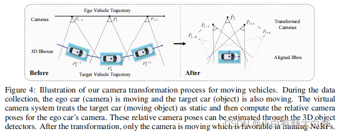
   We now transform the coordinate system by setting the target object’s center as the coordinate system’s origin.
   $${\hat{P}}_i=(P_i{P}_b^{-1}{)}^{-1}=P_b{P}_i^{-1},P^{-1}=\left[\begin{array}{cc}{R}^T& -R^{T}T\\ 0^T& 1\end{array}\right].$$

   And, $P=\left[\begin{array}{cc}R& T\\ 0^T& 1\end{array}\right]$represents the old position of the camera or the target object.

   After the transformation, only the camera is moving which is favorable in training NeRFs.

   How to convert the parameter matrix.

3.2 REPRESENTATION OF STREET SCENES

1. Background scenes

   constrain the whole scene into a bounded range

   

   This part is from mipnerf-360

2. Moving Vehicles

   Compute the dense depth maps for the moving cars as an extra supervision

   • We follow GeoSim (Chen et al., 2021b) to reconstruct coarse mesh from multi-view images and the sparse LiDAR points.

   • After that, a differentiable neural renderer (Liu et al., 2019) is used to render the corresponding depth map with the camera parameter (Section 3.2).

   • The backgrounds are masked during the training by an instance segmentation network (Wang et al., 2020).

   There are three references

3.3 DEPTH SUPERVISION

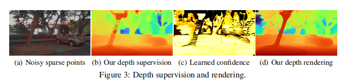
To provide credible depth supervisions from defect LiDAR depths, we first propagate the sparse depths and then construct a confidence map to address the depth outliers（异常值）.

1. LiDAR depth completion

   Use NLSPN (Park et al., 2020) to propagate the depth information from LiDAR points to surrounding pixels.

2. Reprojection confidence

   Measure the accuracy of the depths and locate the outliers.

   The warping operation can be represented as:

   ${\mathbf{X}}_t=\psi ({\psi }^{-1}({\mathbf{X}}_s,P_s),P_t)$

   And we use three features to measure the similarity:

   $${\mathcal{C}}_{\mathrm{rgb}}=1-|{\mathcal{I}}_s-{\hat{\mathcal{I}}}_s|,{\mathcal{C}}_{\mathrm{ssim}}=\mathrm{SSIM}({\mathcal{I}}_s,{\hat{\mathcal{I}}}_s)),{\mathcal{C}}_{\mathrm{vgg}}=1-\Vert {\mathcal{F}}_s-{\hat{\mathcal{F}}}_s\Vert .$$

3. Geometry confidence

   Measure the geometry consistency of the depths and flows across different views.

   The depth:

   $${\mathcal{C}}_{depth}=\gamma (|d_t-{\hat{d}}_t)|/d_s),\gamma (x)=\{\begin{array}{cc}0,& \text{if}x\ge \tau ,\\ 1-x/\tau ,& \text{otherwise}.\end{array}$$

   The flow:

   $${\mathcal{C}}_{flow}=\gamma (\frac{\Vert {\Delta }_{x,y}-f_{s\to t}(x_s,y_s)\Vert }{\Vert {\Delta }_{x,y}\Vert }),{\Delta }_{x,y}=(x_t-x_s,y_t-y_s).$$

4. Learnable confidence combination

   The final confidence map can be learned as $\hat{\mathcal{C}}={\sum }_i{\omega }_i{\mathcal{C}}_i,$ where ${\sum }_i{w}_i=1$ and i ∈ { r g b , s s i m , v g g , d e p t h , f l o w } i \in \{rgb,ssim,vgg,depth,flow\} i∈{rgb,ssim,vgg,depth,flow}

3.4 Loss function

A RGB loss, a depth loss, and an edge-aware smoothness constraint to penalize large variances in depth.
$$\begin{array}{rl}& {\mathcal{L}}_{\mathrm{color}}=\sum _{\mathbf{r}\in \mathcal{R}}\Vert I(\mathbf{r})-\hat{I}(\mathbf{r}){\Vert }_2^2\\ & {\mathcal{L}}_{depth}=\sum \hat{\mathcal{C}}\cdot |\mathcal{D}-\hat{\mathcal{D}}|\\ & {\mathcal{L}}_{smooth}=\sum |{\partial }_x\hat{\mathcal{D}}|{\exp }^{-|{\partial }_{x}I|}+|{\partial }_y\hat{\mathcal{D}}|{\exp }^{-|{\partial }_{y}I|}\\ & {\mathcal{L}}_{\mathrm{total}}={\mathcal{L}}_{\mathrm{color}}+{\lambda }_1{\mathcal{L}}_{depth}+{\lambda }_2{\mathcal{L}}_{smooth}\end{array}$$

4. EXPERIMENTS

0. Dataset: nuScenes and Waymo

• For the foreground vehicles, we extract car crops from nuScenes and Waymo video sequences.
• For the large-scale background scenes, we use scenes with 90∼180 images.
• In each scene, the ego vehicle moves around 10∼40 meters, and the whole scene span more than 200m.

1. Foreground Vehicles

   Different experiments in static vehicles and moving vehicles, compared with Origin-NeRF and GeoSim(the latest non-NeRF car reconstruction method).

   

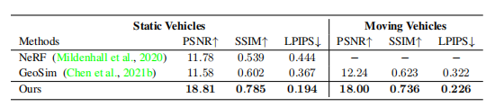
   There are large room for improvement in PSNR

2. Background scenes

   Compared with the state-of-the-art methods Mip-NeRF (Barron et al., 2021), Urban-NeRF (Rematas et al., 2022), and Mip-NeRF 360.
   
   Also, show a 360-degree panorama to emphasize some details:
   

3. BACKGROUND AND FOREGROUND FUSION
   Depth-guided placement and inpainting (e.g. GeoSim Chen et al. (2021b)) and joint NeRF rendering (e.g. GIRAFFE Niemeyer & Geiger (2021)) heavily rely on accurate depth maps and 3D geometry information.
   A new method was used without an introduction?

4. Ablation study
   

   Split into RGB, depth confidence, and smooth loss.

5. Conclusion

In the future, we will use the block merging as proposed in Block-NeRF (Tancik et al., 2022) to learn a larger city-level neural representation

Reference

[1] S-NeRF (ziyang-xie.github.io)