当前位置：首页 > article >正文

Python | basemap空间绘图 | cartopy | geoviews

article 2024/10/19 17:49:15

写在前面

又处理了两周的cmip6数据，真的是daily的资料属实恶心人┗|｀O′|┛ 嗷~~。白天下数据，晚上运行插值脚本。第二天再下数据，再运行插值脚本。两周时间我觉得我的shell编程又进步明显。批量处理数据这一块不能说相当拿手，但是十分熟练了。

峰回路转，抽空整理并复习了一下netcdf官网关于basemap绘制空间分布图的几种类型，为后续绘图做准备，发现basemap画图有他好用的道理，确实相比cartopy要方便不少。

同时发现了两个有意思的库，geoviews以及holoviews可以更方便快捷的绘制各自空间分布图。

下面基于sst数据对不同投影进行简单演示：

basemap

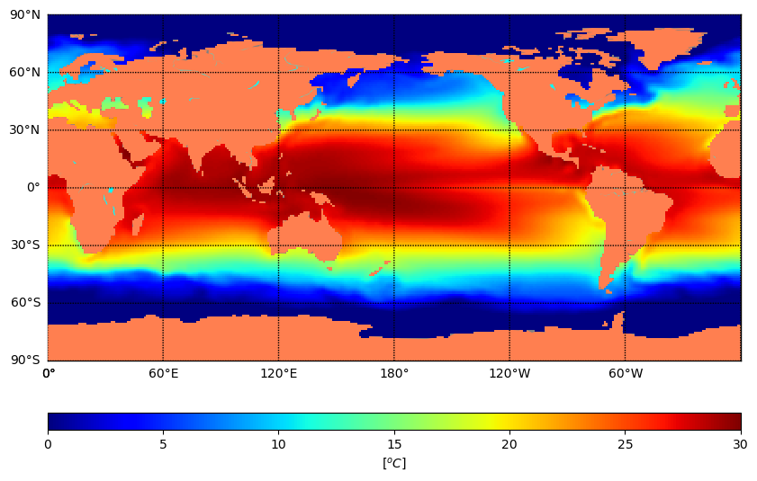
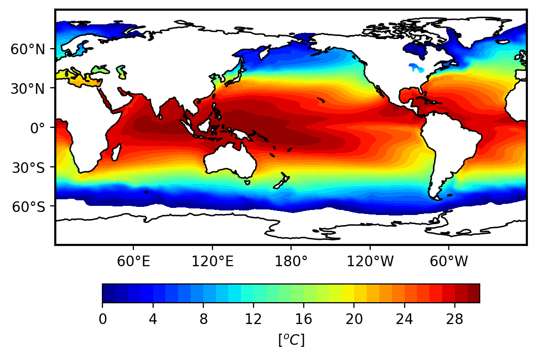
等距圆柱投影


m = Basemap(projection='cyl', lon_0=180,resolution='c')
m.fillcontinents(color='coral',lake_color='aqua')
m.drawmapboundary(fill_color='Gray', zorder=0)
m.drawparallels(np.arange(-90.,99.,30.), labels=[1,0,0,0])
m.drawmeridians(np.arange(0.,360.,60.), labels=[0,0,0,1])
h = m.pcolormesh(lons, lats, sst_mean,latlon=True, vmin=0.0, vmax=30.0,cmap='jet')
m.colorbar(h, location='bottom', pad="15%", label='[$^oC$]')

cyl

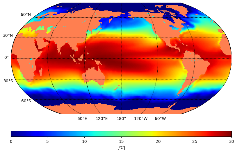
Robin


m = Basemap(projection='robin', lon_0=180,resolution='c')
m.fillcontinents(color='coral',lake_color='aqua')
m.drawmapboundary(fill_color='Gray', zorder=0)
m.drawparallels(np.arange(-90.,99.,30.), labels=[1,0,0,0])
m.drawmeridians(np.arange(0.,360.,60.), labels=[0,0,0,1])
h = m.pcolormesh(lons, lats, sst_mean,latlon=True,cmap='jet',vmin=0.0, vmax=30.0,)
m.colorbar(h, location='bottom', pad="15%", label='[$^oC$]')

robin

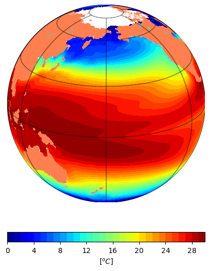
Full Disk Orthographic Projection


m = Basemap(projection='ortho', lon_0=-180, lat_0=20, resolution='c')
m.fillcontinents(color='coral', lake_color='aqua')
m.drawparallels(np.arange(0.,120.,30.))
m.drawmeridians(np.arange(0.,420.,60.))

h = m.contourf(lons, lats, sst_mean, latlon=True, cmap='jet',levels=np.linspace(0,30,31))
m.colorbar(h, location='bottom', pad="15%", label='[$^oC$]')

ortho

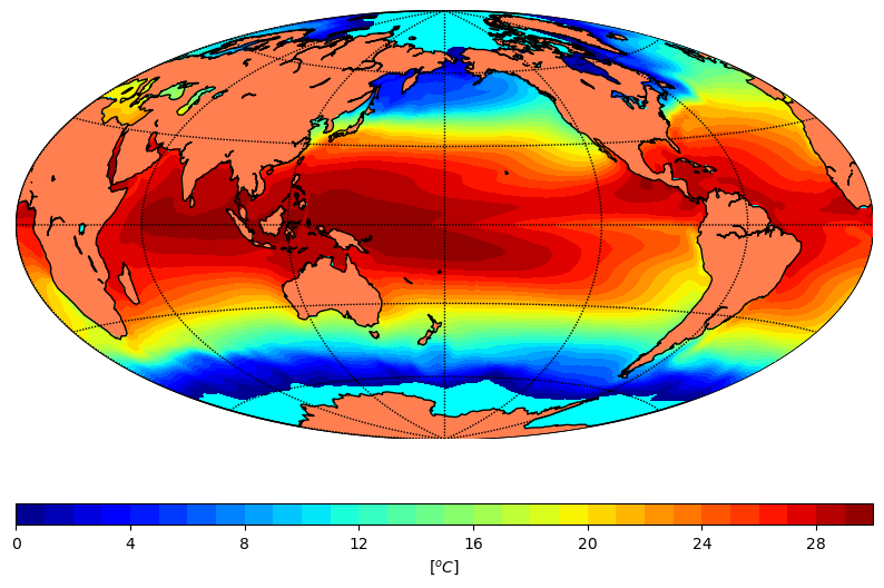
Hammer Projection

m = Basemap(projection='hammer', lon_0=180)
m.drawcoastlines()
m.fillcontinents(color='coral',lake_color='aqua')
# draw parallels and meridians.
m.drawparallels(np.arange(-90.,120.,30.))
m.drawmeridians(np.arange(0.,420.,60.))
m.drawmapboundary(fill_color='aqua')
h = m.contourf(lons, lats, sst_mean,latlon=True, levels=np.linspace(0,30,31),cmap='jet')
m.colorbar(h, location='bottom', pad="15%", label='[$^oC$]')

hammer

cartopy

等间距投影，这个用的最多，就简单给个封装的常用代码，方便后续直接使用

import cartopy.crs as ccrs
def set_ax(ax, lon, lat, data,proj):
    from cartopy.mpl.ticker import LongitudeFormatter, LatitudeFormatter
    import matplotlib.ticker as mticker
    import matplotlib.ticker as ticker
    
    xstep, ystep = 6, 6
    box = [0, 360, -90, 90]
    # ax.set_xlim(box[0], box[1])
    # ax.set_ylim(box[2], box[3])
    ax.set_xticks(np.linspace(box[0], box[1], int((box[1] - box[0]) / xstep) + 1), crs=proj)
    ax.set_yticks(np.linspace(box[2], box[3], int((box[3] - box[2]) / ystep) + 1), crs=proj)
    ax.xaxis.set_major_formatter(LongitudeFormatter())
    ax.yaxis.set_major_formatter(LatitudeFormatter())
    ax.xaxis.set_major_locator(mticker.MultipleLocator(60))
    ax.yaxis.set_major_locator(mticker.MultipleLocator(30))
    ax.spines[['right', 'left', 'top', 'bottom']].set_linewidth(1.5)
    ax.spines[['right', 'left', 'top', 'bottom']].set_visible(True)
    cf = ax.contourf(lons, lats, data, cmap='jet', transform=proj, levels=np.linspace(0, 30, 31))
    ax.coastlines()
    cbar = plt.colorbar(cf, ax=ax, orientation='horizontal', pad=0.1,shrink=0.8)
    cbar.set_label('[$^oC$]')
    
fig, ax = plt.subplots(figsize=(6, 5),dpi=200,
                        subplot_kw={'projection': ccrs.PlateCarree(central_longitude=180)})

set_ax(ax,lon,lat,sst_mean,proj=ccrs.PlateCarree(central_longitude=0))


plt.show()

PlateCarree

geoviews && holoviews

https://geoviews.org/index.html
https://holoviews.org/

这两个库挺好玩的，安装也很方便

conda install holoviews,geoviews

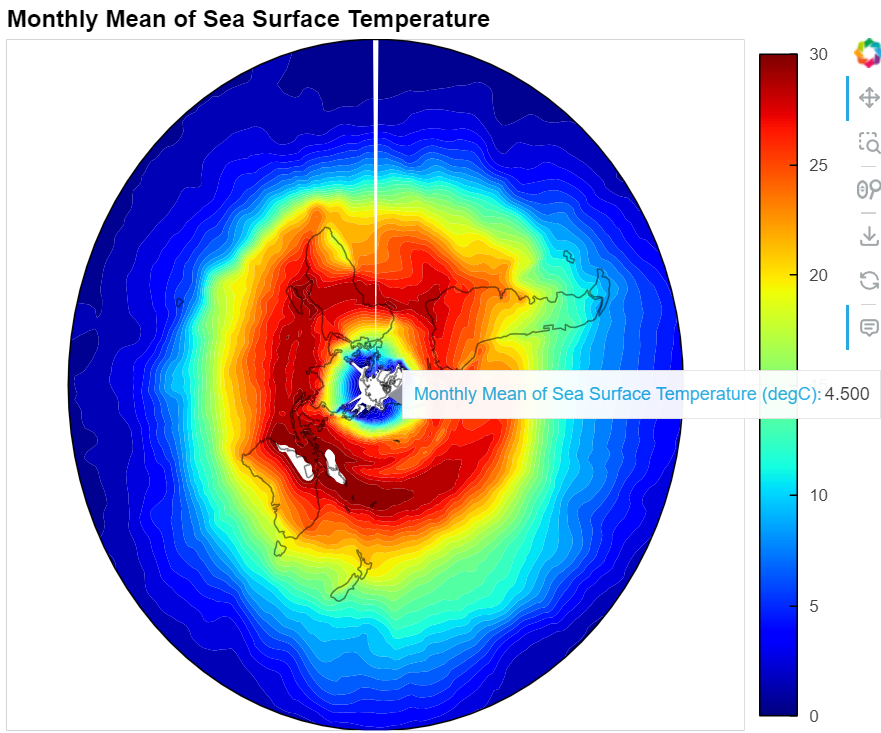
通过一段核心代码，就可以实现任意投影的转换;缺点是细节不太美观，对于科研绘图还是需要自己仔细调整，用来娱乐一下挺好玩的。


def plot(variable='sst', projection=ccrs.PlateCarree(), width=600, height=500, levels=10, 
         cmap='Spectral', global_extent=True, **kwargs):
    
    # from cartopy.mpl.ticker import LongitudeFormatter, LatitudeFormatter
    """Plot filled countour plots for different cartopy projections while using hvplot/holoviews/geoviews"""
    long_name = ds[variable].long_name
    print(long_name)
    units = ds[variable].units

    spacing = 80 * " "
    title = f'{long_name} {spacing} {units}'
    p = ds.hvplot(x='lon', y='lat', z=variable, projection=projection,
                width=width, height=height, cmap=cmap, dynamic=False, 
                kind='contourf', levels=levels, title=title, 
                legend='bottom', global_extent=global_extent,
                xticks=np.linspace(-180, 180, 13), 
                yticks=np.linspace(-90, 90, 7), 
                xlim=(-180, 180), ylim=(-90, 90),  

                ylabel=f'{ds.lat.long_name}[{ds.lat.units}]', 
                xlabel=f'{ds.lon.long_name}[{ds.lon.units}]',
                **kwargs
    ) * gv.feature.coastline
    p.opts(
        xticks=[(x, LongitudeFormatter()(x)) for x in np.linspace(-180, 180, 13)],
        yticks=[(y, LatitudeFormatter()(y)) for y in np.linspace(-90, 90, 7)]
    )
    return p

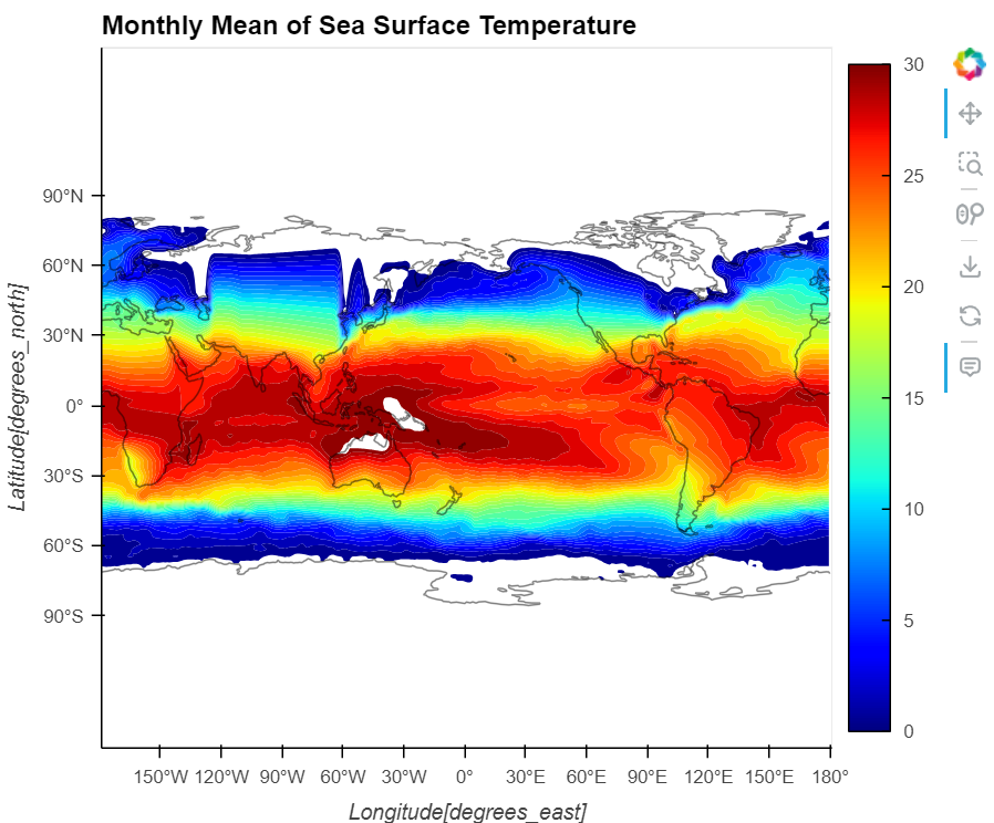
PlateCarree

AlbersEqualArea

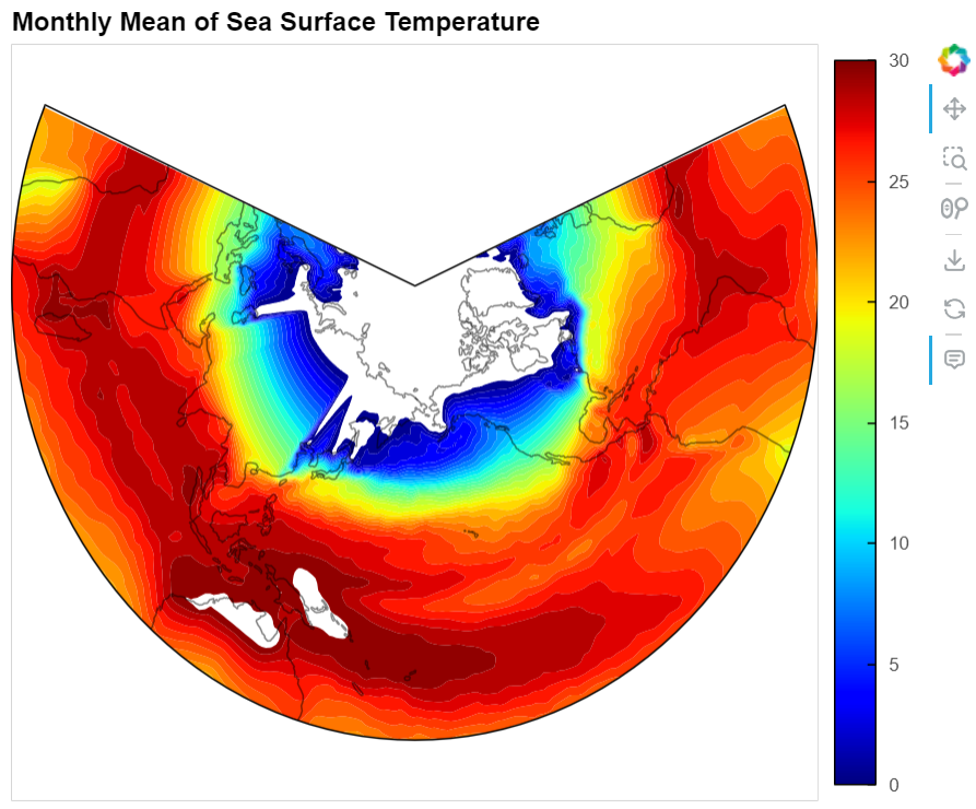
LambertConformal

Robinson

SouthPolarStereo

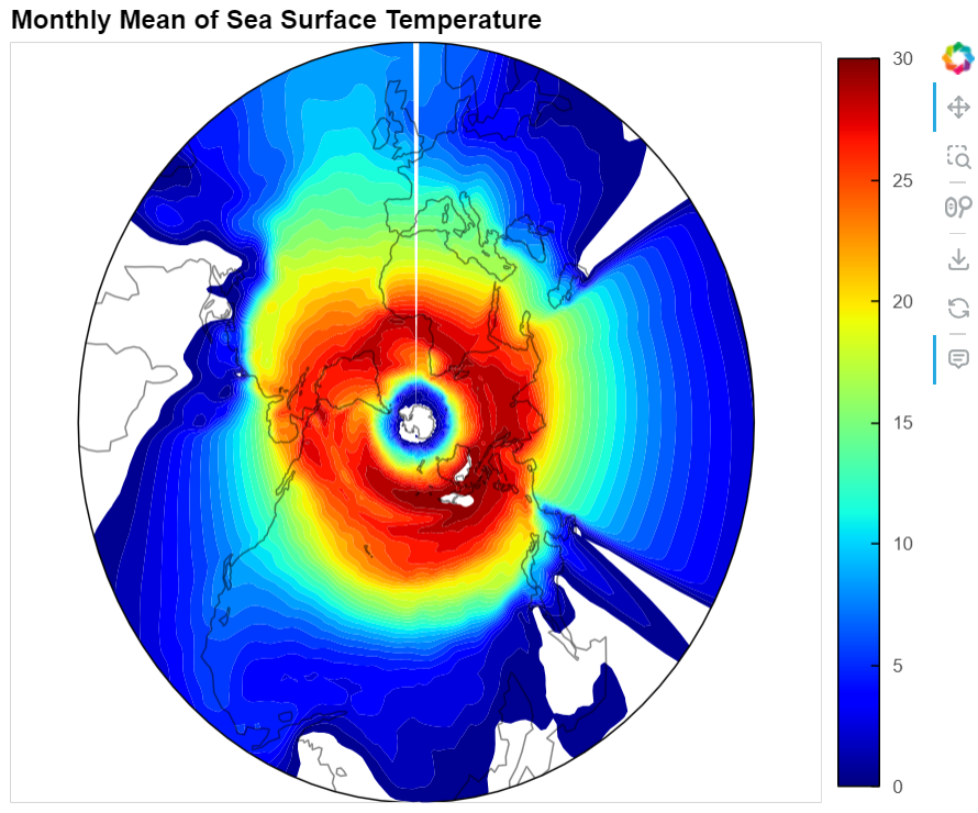
NorthPolarStereo

数据还是直接上传的sst数据，代码也放到了GitHub上，可以自己替换数据体验一下。

https://github.com/Blissful-Jasper/jianpu_record

https://ncar-hackathons.github.io/visualization/cartopy-basics.html

https://ncar-hackathons.github.io/visualization/examples/cartopy_map_projections.html

http://unidata.github.io/netcdf4-python/

查看全文

http://www.kler.cn/news/356163.html