深入理解全连接层：从线性代数到 PyTorch 中的 nn.Linear 和 nn.Parameter

这篇文章会从基础的一个数学概念到对应的代码实现，你将了解到：

• 为什么nn.Parameter()接受$(\text{out\_features},\text{in\_features})$作为参数？
• 为什么不是torch.matmul(self.weight, x) + self.bias？
• 如何使用torch.matmul()，@或 F.linear() 去等价地实现nn.Linear()的输出。

数学概念（全连接层，线性层）

线性变化是数学中一个基础的概念，它描述了如何通过线性变换将输入映射到输出。在线性代数中，线性变化通常表示为矩阵乘法。在神经网络中，线性层的核心就是实现这样的矩阵运算。

数学公式：

给定一个输入向量 $\mathbf{x}\in {\mathbb{R}}^n$ 和一个输出向量 $\mathbf{y}\in {\mathbb{R}}^m$，线性变化通过矩阵 $\mathbf{W}\in {\mathbb{R}}^{m\times n}$ 和偏置项 $\mathbf{b}\in {\mathbb{R}}^m$ 进行变换，其公式为：
$$\mathbf{y}=\mathbf{Wx}+\mathbf{b}$$

• $\mathbf{W}$：是权重矩阵，维度为 $m\times n$，它决定了输入向量如何线性变换到输出空间；
• $\mathbf{x}$：是输入向量，维度为 $n$，表示特征数据；
• $\mathbf{b}$：是偏置向量，维度为 $m$，用来调整线性变换的输出；
• $\mathbf{y}$：是输出向量，维度为 $m$，是变换后的结果。

例子：

如果输入向量 $\mathbf{x}$ 有 3 个特征，输出向量 $\mathbf{y}$ 有 2 个特征，则权重矩阵 $\mathbf{W}$ 的形状为 $2\times 3$。假设：
$$\mathbf{W}=\left[\begin{array}{ccc}1& 2& 3\\ 4& 5& 6\end{array}\right],\mathbf{x}=\left[\begin{array}{c}1\\ 2\\ 3\end{array}\right],\mathbf{b}=\left[\begin{array}{c}0\\ 1\end{array}\right]$$
线性变换计算为：
$$\mathbf{y}=\mathbf{Wx}+\mathbf{b}=\left[\begin{array}{ccc}1& 2& 3\\ 4& 5& 6\end{array}\right]\left[\begin{array}{c}1\\ 2\\ 3\end{array}\right]+\left[\begin{array}{c}0\\ 1\end{array}\right]=\left[\begin{array}{c}14\\ 32\end{array}\right]+\left[\begin{array}{c}0\\ 1\end{array}\right]=\left[\begin{array}{c}14\\ 33\end{array}\right]$$
矩阵运算过程：
$$\left[\begin{array}{ccc}1& 2& 3\\ 4& 5& 6\end{array}\right]\left[\begin{array}{c}1\\ 2\\ 3\end{array}\right]=\left[\begin{array}{c}(1\times 1)+(2\times 2)+(3\times 3)\\ (4\times 1)+(5\times 2)+(6\times 3)\end{array}\right]=\left[\begin{array}{c}14\\ 32\end{array}\right]$$

nn.Linear()

nn.Linear() 会自动创建一个权重矩阵（Weight）和偏置项（Bias），并将它们应用到输入上。

代码示例：

import torch
import torch.nn as nn

# 定义一个输入为3，输出为2的线性层
linear_layer = nn.Linear(3, 2)

# 打印权重矩阵和偏置项
print("权重矩阵 W:")
print(linear_layer.weight)

print("偏置项 b:")
print(linear_layer.bias)

# 模拟输入向量
input_vector = torch.tensor([1.0, 2.0, 3.0])
output_vector = linear_layer(input_vector)
print("输出向量 y:")
print(output_vector)

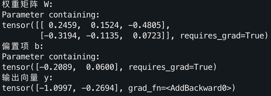
在这里，nn.Linear(3, 2) 创建了一个 2×3 的权重矩阵和一个 2 维的偏置向量。通过 linear_layer(input_vector)，可以直接获得输入向量经过线性变换后的输出。

nn.Parameter()

在 PyTorch 中，nn.Linear() 自动处理了权重和偏置项的初始化和更新，但有时你可能希望对这些参数自定义一些操作，比如 LoRA。这时，我们可以使用 nn.Parameter() 来自定义权重和偏置，其实 nn.Linear() 本身就是使用的nn.Parameter()，感兴趣的话可以看官方源码。

以自定义线性层为例：

class CustomLinearLayer(nn.Module):
    def __init__(self, input_dim, output_dim):
        super(CustomLinearLayer, self).__init__()
        # 使用 nn.Parameter 手动定义权重和偏置
        self.weight = nn.Parameter(torch.randn(output_dim, input_dim))
        self.bias = nn.Parameter(torch.randn(output_dim))

    def forward(self, x):
        # 手动实现线性变换 y = Wx + b
        return torch.matmul(x, self.weight.T) + self.bias

# 使用自定义的线性层
custom_layer = CustomLinearLayer(3, 2)
output = custom_layer(input_vector)
print(output)

在看完代码后，你可能会产生两个疑惑：

Q

1. 为什么 self.weight 的权重矩阵 shape 使用$(\text{out\_features},\text{in\_features})$而不是$(\text{in\_features},\text{out\_features})$?

这正是我写这篇博客的原因，接下来我们详细解释这个问题。

让我们重新使用$\text{in\_features}$和$\text{out\_features}$来重现之前的数学定义：

对于输入向量 $\mathbf{x}\in {\mathbb{R}}^{\text{in\_features}}$，全连接层的输出为：

$$\mathbf{y}=W\mathbf{x}+\mathbf{b}$$

其中：

• $W\in {\mathbb{R}}^{\text{out\_features}\times \text{in\_features}}$ 是权重矩阵，
• $\mathbf{b}\in {\mathbb{R}}^{\text{out\_features}}$ 是偏置项。

在线性变换中，输入向量 $\mathbf{x}$ 的维度是 $\text{in\_features}$，而输出向量 $\mathbf{y}$ 的维度是 $\text{out\_features}$。根据矩阵乘法的规则，要将输入 $\mathbf{x}$ 映射到输出 $\mathbf{y}$，权重矩阵 $W$ 的形状应该是 $(\text{out\_features},\text{in\_features})$，因为矩阵乘法中$W\mathbf{x}$的维度要求是：

$$(\text{out\_features}\times \text{in\_features})\times (\text{in\_features}\times 1)=(\text{out\_features}\times 1)$$

这保证了输出 $\mathbf{y}$ 的维度是 $\text{out\_features}$。

如果权重矩阵的形状是 $(\text{in\_features},\text{out\_features})$，矩阵乘法的维度将不匹配，无法实现线性变换。

现在是不是感觉清晰了？不要 nn.Linear(in_feature, out_feature) 用多了就将权重矩阵当作是$(\text{in\_features},\text{out\_features})$遗忘了线性代数的概念，数学才是这一切的基石。

2. 为什么是torch.matmul(x, self.weight.T) + self.bias 而不是torch.matmul(self.weight, x) + self.bias?

主要原因还是在于 输入张量 x 的形状 和 矩阵乘法规则。

一般来说，模型的输入 x 实际上并不是 $(\text{in\_features},1)$，而是 $(\text{batch\_size},\text{in\_features})$，而权重矩阵 self.weight 的形状是 $(\text{out\_features},\text{in\_features})$​，我们需要实现的线性变换是：
$$y=Wx+b$$
根据矩阵乘法规则，第一个矩阵的列数必须等于第二个矩阵的行数，这意味着我们不能直接计算 torch.matmul(self.weight, x)，因为这样会导致维度不匹配：

• self.weight 形状为 $(\text{out\_features},\text{in\_features})$，x 形状为 $(\text{batch\_size},\text{in\_features})$。
• torch.matmul(self.weight, x) 的维度计算规则将要求 x 的形状为 $(\text{in\_features},\text{batch\_size})$，但这与模型的输入不匹配。

因此，正确的矩阵乘法应该是 torch.matmul(x, self.weight.T)，其中 self.weight.T 表示 self.weight 的转置矩阵，此时的形状为 $(\text{in\_features},\text{out\_features})$。

这样，torch.matmul(x, self.weight.T) 的维度计算为：

$$(\text{batch\_size},\text{in\_features})\times (\text{in\_features},\text{out\_features})=(\text{batch\_size},\text{out\_features})$$

这就得到了正确的输出形状$(\text{batch\_size},\text{out\_features})$。

3. 为什么不直接设置self.weight = nn.Parameter(torch.randn(input_dim, output_dim))？

这样不就可以不转置直接使用torch.matmul(x, self.weight)了吗？的确如此，或许是因为 $(\text{out\_features},\text{in\_features})$ 对于矩阵运算 $W\mathbf{x}$ 来讲更符合直觉吧。

计算过程的细分：torch.matmul() vs @ 运算符

在 PyTorch 中，torch.matmul() 用于实现矩阵乘法，而 @ 是其简洁的符号形式，是 Python 的语法糖，二者在功能上是等价的。

示例代码：

import torch

# 定义权重矩阵 W 和输入向量 input_vector
W = torch.tensor([[1.0, 2.0, 3.0], [4.0, 5.0, 6.0]])
input_vector = torch.tensor([1.0, 2.0, 3.0])

# 使用 torch.matmul 实现矩阵乘法
result1 = torch.matmul(W, input_vector)

# 使用 @ 运算符
result2 = W @ input_vector

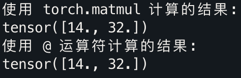
print("使用 torch.matmul 计算的结果:")
print(result1)

print("使用 @ 运算符计算的结果:")
print(result2)

结果：

使用 F.linear()

PyTorch 提供了 F.linear() 作为函数式接口，它与 nn.Linear() 类似，但不需要创建一个线性层对象。F.linear() 可以接受线性层的权重和偏置作为输入。

示例代码：

import torch.nn.functional as F

# 使用 F.linear 进行线性变换
output = F.linear(input_vector, linear_layer.weight, linear_layer.bias)
print(output)