【机器学习】使用Numpy实现神经网络训练全流程
文章目录
- 网络搭建
- 前向传播
- 反向传播
- 损失计算
- 完整代码
曾经在面试一家大模型公司时遇到的面试真题,当时费力写了一个小时才写出来,自然面试也挂了。后来复盘,发现反向传播掌握程度还是太差,甚至连梯度链式传播法则都没有弄明白。
网络搭建
这里我们以训练 全连接神经网络 为例,也就是输入层,隐藏层和输出层都是 全连接层,激活函数选择Relu函数。
- 构造Linear层来实现全连接层,其中权重参数 w w w和偏执参数 b i a s bias bias分别使用随机初始化和零初始化
- Relu激活函数没有可学习参数
- 整个网络写成MLP类,并设置参数控制中间隐藏层的个数
class Relu:
    ''' relu activation function
    '''
    def forward(self, x):
        self.x = x
        return np.maximum(0, x)

class LinearLayer:
    def __init__(self, input_c, output_c):
        # y = x @ w + b
        # self.w = np.random.rand(input_c, output_c)
        self.w = np.random.rand(input_c, output_c) * 0.001 # 这里乘上0.001是为了防止结果太大,梯度爆炸
        self.b = np.zeros(output_c)

class MLP:
    def __init__(self, input_c, hidden_c, output_c, layers_num):
        self.layers = []

        # 初始化网络第一层
        self.layers.append(LinearLayer(input_c, hidden_c))
        self.layers.append(Relu())

        # 初始化网络中间层
        for i in range(layers_num - 2):
            self.layers.append(LinearLayer(hidden_c, hidden_c))
            self.layers.append(Relu())

        # 初始化网络最后一层,注意,最后一层没有relu激活函数
        self.layers.append(LinearLayer(hidden_c, output_c))
前向传播
前向传播部分,主要包括 Linear层的前向,Relu激活函数的前向,以及MLP类的前向:
- Relu激活函数:前向就是和0比较大小,大于零的保留,小于零的都置为0
- Linear层:前向计算公式就是线性回归方程,要注意计算时维度需要对齐
- MLP类:逐层调用前向传播函数
class Relu:
    ''' relu activation function
    '''
    def forward(self, x):
        self.x = x
        return np.maximum(0, x)

class LinearLayer:
    def __init__(self, input_c, output_c):
        # y = x @ w + b
        # self.w = np.random.rand(input_c, output_c)
        self.w = np.random.rand(input_c, output_c) * 0.001 # 这里乘上0.001是为了防止结果太大,梯度爆炸
        self.b = np.zeros(output_c)

    def forward(self, x):
        self.x = x # 这里保存输入,为了后续在反向传播中计算梯度
        # y = x @ w + b
        return np.dot(x, self.w) + self.b

class MLP:
    def __init__(self, input_c, hidden_c, output_c, layers_num):
        self.layers = []

        # 初始化网络第一层
        self.layers.append(LinearLayer(input_c, hidden_c))
        self.layers.append(Relu())

        # 初始化网络中间层
        for i in range(layers_num - 2):
            self.layers.append(LinearLayer(hidden_c, hidden_c))
            self.layers.append(Relu())

        # 初始化网络最后一层,注意,最后一层没有relu激活函数
        self.layers.append(LinearLayer(hidden_c, output_c))


    def forward(self, x):
        res = x
        for layer in self.layers:
            res = layer.forward(res)
        return res
反向传播
前向的输出,变为反向的输入
梯度,就是多元函数对某个变量的偏导数(变化最快的方向)
梯度下降法更新参数,就是朝着梯度的反方向更新参数
参数的梯度,意思是 损失函数对这个参数的梯度,根据求导的链式法则,可以表示为逐层求导乘积的形式
同前向一样,反向传播部分,也包括 Linear层的反向,Relu激活函数的反向,以及MLP类的反向:
- Relu激活函数:大于0时导数为1,小于等于0时导数为0。同时由于没有可学习参数,所以只需要回传输入的梯度值即可
- MLP类:由于是反向传播,所以起点就是 损失函数 对于 MLP最后一层的输出 的梯度值,然后从最后一层向前,逐层 回传 梯度值
- Linear层:由于存在可学习参数需要去更新,因此不仅需要计算输入的梯度,还需要计算两个可学习参数 w w w和 b i a s bias bias的梯度,然后更新参数
class Relu:
    ''' relu activation function
    '''
    def forward(self, x):
        self.x = x
        return np.maximum(0, x)

    def backward(self, grad_output, lr):
        # 这里的lr没有用到,但是为了保持参数接口的一致性,还是保留了
        return grad_output * (self.x > 0) # relu函数的一阶导数,大于0部分为1,小于0部分为0

class LinearLayer:
    def __init__(self, input_c, output_c):
        # y = x @ w + b
        # self.w = np.random.rand(input_c, output_c)
        self.w = np.random.rand(input_c, output_c) * 0.001 # 这里乘上0.001是为了防止结果太大,梯度爆炸
        self.b = np.zeros(output_c)

    def forward(self, x):
        self.x = x # 这里保存输入,为了后续在反向传播中计算梯度
        # y = x @ w + b
        return np.dot(x, self.w) + self.b

    def backward(self, grad_output, lr):
        # linear层的梯度计算,涉及三个参数,x,w,b,为 dx, dw, db
        # 其中,dw和db是为了更新w和b
        # dx是为了计算下一层的梯度,链式法则

        # y = x @ w + b
        # dl / dx = dl / dy * dy / dx = grad_output * w
        # 这里要注意矩阵的维度要对齐
        grad_input = np.dot(grad_output, self.w.T)

        # dl / dw = dl / dy * dy / dw = grad_output * x
        # 这里要注意矩阵的维度要对齐
        w_grad = np.dot(self.x.T, grad_output)

        b_grad = np.sum(grad_output, axis=0)

        # 更新w和b的参数
        self.w -= lr * w_grad
        self.b -= lr * b_grad

        return grad_input

class MLP:
    def __init__(self, input_c, hidden_c, output_c, layers_num):
        self.layers = []

        # 初始化网络第一层
        self.layers.append(LinearLayer(input_c, hidden_c))
        self.layers.append(Relu())

        # 初始化网络中间层
        for i in range(layers_num - 2):
            self.layers.append(LinearLayer(hidden_c, hidden_c))
            self.layers.append(Relu())

        # 初始化网络最后一层,注意,最后一层没有relu激活函数
        self.layers.append(LinearLayer(hidden_c, output_c))


    def forward(self, x):
        res = x
        for layer in self.layers:
            res = layer.forward(res)
        return res

    def backward(self, grad_output, lr):
        grad = grad_output

        # 倒序遍历每一层,反向传播,计算每一层梯度
        # for layer in reversed(self.layers):
        for layer in self.layers[::-1]:
            grad = layer.backward(grad, lr)

        return grad
损失计算
这里为了简化操作,使用MSE均方误差函数,作为损失函数:
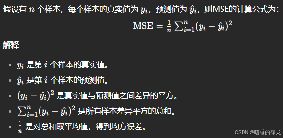
然后,计算损失loss对模型最后一层输出的梯度:
l
g
r
a
d
=
2
∗
(
y
−
y
^
)
l_{grad}=2*(y-\hat{y})
lgrad=2∗(y−y^),然后,将
l
g
r
a
d
l_{grad}
lgrad作为模型反向传播的起点,逐层回传梯度并使用梯度下降法更新参数。
完整代码
import numpy as np

class Relu:
    ''' relu activation function
    '''
    def forward(self, x):
        self.x = x
        return np.maximum(0, x)

    def backward(self, grad_output, lr):
        # 这里的lr没有用到,但是为了保持参数接口的一致性,还是保留了
        return grad_output * (self.x > 0) # relu函数的一阶导数,大于0部分为1,小于0部分为0

class LinearLayer:
    def __init__(self, input_c, output_c):
        # y = x @ w + b
        # self.w = np.random.rand(input_c, output_c)
        self.w = np.random.rand(input_c, output_c) * 0.001 # 这里乘上0.001是为了防止结果太大,梯度爆炸
        self.b = np.zeros(output_c)

    def forward(self, x):
        self.x = x # 这里保存输入,为了后续在反向传播中计算梯度
        # y = x @ w + b
        return np.dot(x, self.w) + self.b

    def backward(self, grad_output, lr):
        # linear层的梯度计算,涉及三个参数,x,w,b,为 dx, dw, db
        # 其中,dw和db是为了更新w和b
        # dx是为了计算下一层的梯度,链式法则

        # y = x @ w + b
        # dl / dx = dl / dy * dy / dx = grad_output * w
        # 这里要注意矩阵的维度要对齐
        grad_input = np.dot(grad_output, self.w.T)

        # dl / dw = dl / dy * dy / dw = grad_output * x
        # 这里要注意矩阵的维度要对齐
        w_grad = np.dot(self.x.T, grad_output)

        b_grad = np.sum(grad_output, axis=0)

        # 更新w和b的参数
        self.w -= lr * w_grad
        self.b -= lr * b_grad

        return grad_input

class MLP:
    def __init__(self, input_c, hidden_c, output_c, layers_num):
        self.layers = []

        # 初始化网络第一层
        self.layers.append(LinearLayer(input_c, hidden_c))
        self.layers.append(Relu())

        # 初始化网络中间层
        for i in range(layers_num - 2):
            self.layers.append(LinearLayer(hidden_c, hidden_c))
            self.layers.append(Relu())

        # 初始化网络最后一层,注意,最后一层没有relu激活函数
        self.layers.append(LinearLayer(hidden_c, output_c))


    def forward(self, x):
        res = x
        for layer in self.layers:
            res = layer.forward(res)
        return res

    def backward(self, grad_output, lr):
        grad = grad_output

        # 倒序遍历每一层,反向传播,计算每一层梯度
        # for layer in reversed(self.layers):
        for layer in self.layers[::-1]:
            grad = layer.backward(grad, lr)

        return grad

if __name__ == '__main__':
    input_data = np.random.rand(2, 8)
    input_c = 8
    hidden_c = 16
    output_c = 3
    layers = 5
    target = np.random.rand(2, 3)

    mlp_model = MLP(input_c, hidden_c, output_c, layers)

    # print(mlp_model.layers)

    for i in range(10):
        print(f'[Epoch: {i} / 100]', end='   ')
        res = mlp_model.forward(input_data)

        # 计算损失loss,这里使用mse,均方误差函数
        loss = ((res - target) ** 2).mean()

        # 损失对于最后一层输出res的梯度
        loss_grad = 2 * (res - target)

        # 反向传播,计算每一层梯度
        mlp_model.backward(loss_grad, lr=0.1)

        print(f'[loss: {loss}]')
输出结果:
[Epoch: 0 / 100]   [loss: 0.7094113331502839]
[Epoch: 1 / 100]   [loss: 0.2770589775342763]
[Epoch: 2 / 100]   [loss: 0.12141369105814748]
[Epoch: 3 / 100]   [loss: 0.06538216434144564]
[Epoch: 4 / 100]   [loss: 0.04521136910150728]
[Epoch: 5 / 100]   [loss: 0.037950191234703855]
[Epoch: 6 / 100]   [loss: 0.03533631186000425]
[Epoch: 7 / 100]   [loss: 0.03439537638899603]
[Epoch: 8 / 100]   [loss: 0.034056663841438094]
[Epoch: 9 / 100]   [loss: 0.033934736564443235]